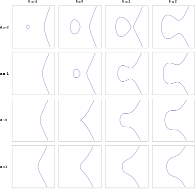
Refer To The Diagram To The Right Curve G Approaches Curve F Because
H average fixed cost curve. Refer to the above diagram.
 Avoid Overfitting By Early Stopping With Xgboost In Python
Identify the curves in the diagram.

Refer to the diagram to the right curve g approaches curve f because. Refer to figure m2 6 curve g approaches curve f school texas am university. Home study business economics economics questions and answers refer to figure 11 4. Refer to figure 10 4.
Curve g approaches curve f because 10 11if the marginal cost curve is below the average variable cost curve then 11 12if when a firm doubles all its inputs its average cost of production increases then production displays adiseconomies of scale. Curve g approaches curve f because a marginal cost is above average variable costs. G average variable cost curve.
In a diagram that shows the marginal product of labor on the. Identify the curves in the diagram. E marginal cost curve.
Answer aproduction possibilities curve indicating constant opportunity costs. Introduction to microeconomics final exam sample questions multiple choice. Shift curve a to the left and shift curve b downward.
Curve g approaches curve f because a fixed cost falls as capacity rises. Curve a shifts to the right. B total cost falls as more and more is produced.
Course title econ 202. Identify the curves in the diagram. Refer to the above diagrams.
9 10 refer to figure 11 4. As will be seen in fig. E average fixed cost curve.
Cdemand curve indicating that the quantity of consumer goods demanded increases as the price of capital falls. 90 20 18 out of 20 people found this. F average total cost curve.
C average fixed cost falls as output rises. Identify the curves in the diagram. A firm finds that at its mrmc output its tc 1000 tvc 800 tfc 200 and total revenue is 900.
Shift curve a to the right and shift curve b upward. Bproduction possibilities curve indicating increasing opportunity costs. Leave curve a in place but shift curve b downward.
41 9 42 refer to figure 11 1. The demand curve in a perfectly competitive industry is while the demand curve to a single firm in that industry is. Curve b is a.
88 the left hand portion of an indifference curve of the perfect complementary goods is a vertical straight line which indicates that an infinite amount of y is necessary to substitute one unit of x and the right hand portion of the indifference curve is a horizontal straight line which means that an infinite amount of x is necessary to substitute one unit of y. Leave curve a in place but shift curve b upward.
 Fragility Curves For Stone Left And Brick Masonry Right
 Econ 150 Microeconomics
 Extended Master Curve Showing The Scaled Elastic Modulus Of The
 Spontaneous Droplets Gyrating Via Asymmetric Self Splitting On
 Elliptic Curve Wikipedia
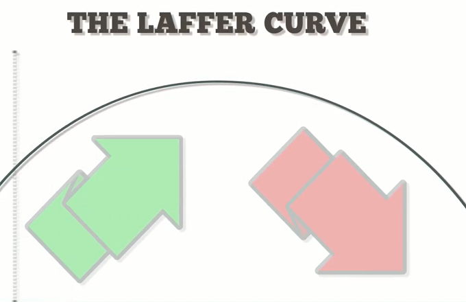 Laffer Curve
Notched Plate With Hole Stag And Mon Ls Load Displacement Curves In
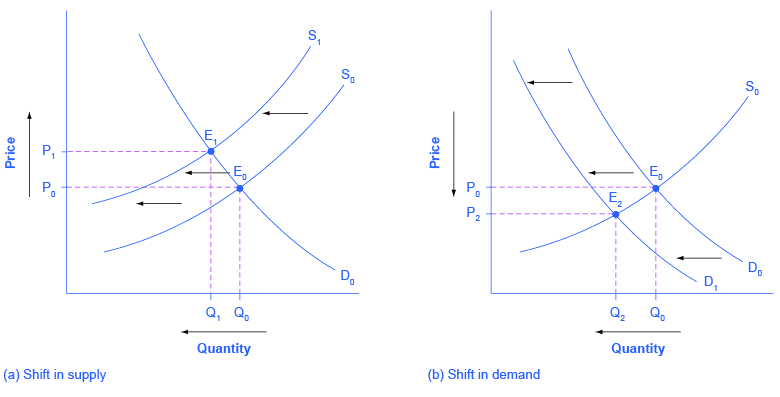 Changes In Equilibrium Price And Quantity The Four Step Process
 The Economy Unit 10 Banks Money And The Credit Market
 The Lorenz Curve And Gini Coefficient Intelligent Economist
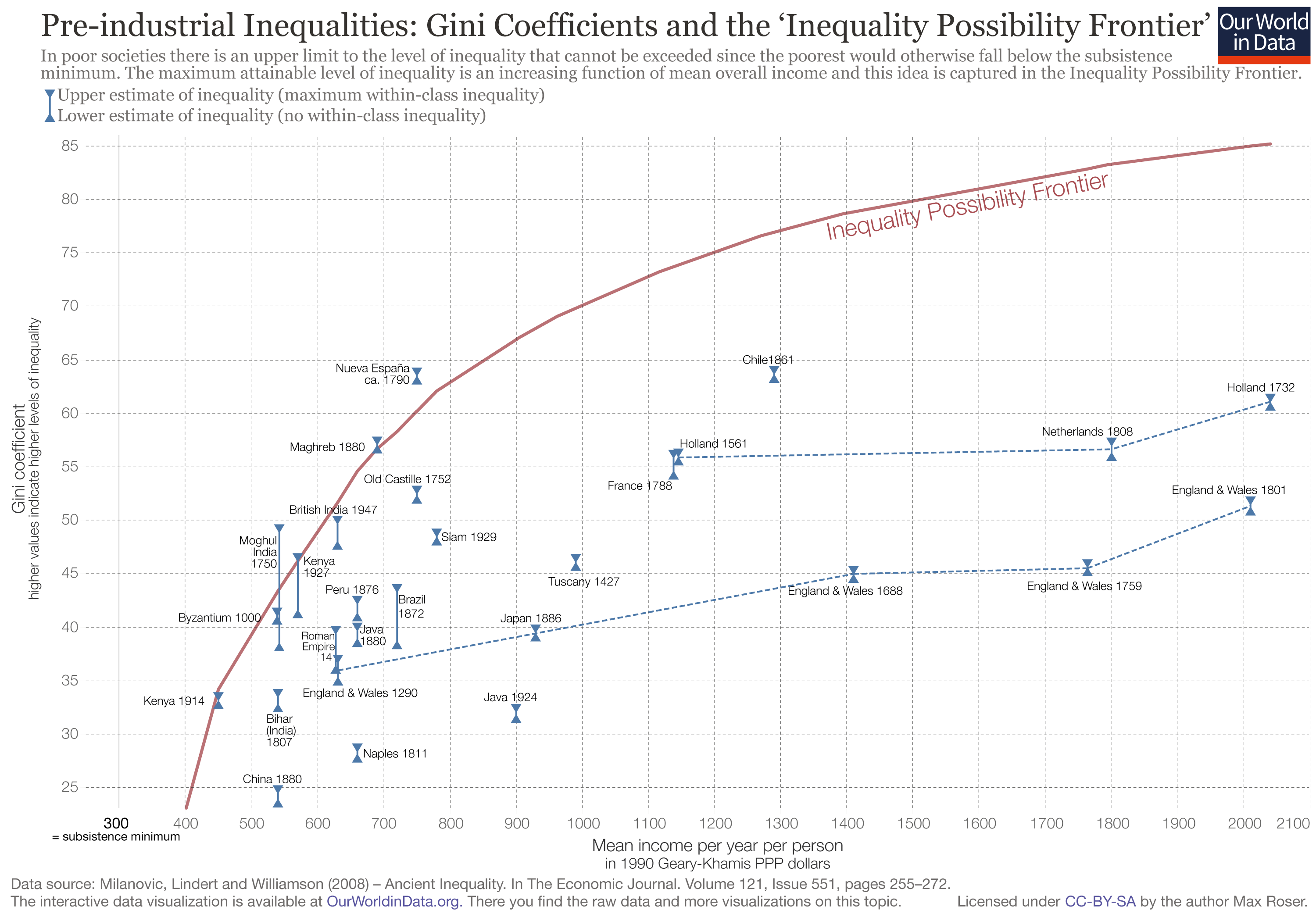 Income Inequality Our World In Data

 The Economy Unit 10 Banks Money And The Credit Market
 Gain Curves Depicting The Pulse Rate Mn As A Function Of The Driving

 The Economy Unit 10 Banks Money And The Credit Market
 Chronic Obstructive Pulmonary Disease Copd Practice Essentials
0 Response to "Refer To The Diagram To The Right Curve G Approaches Curve F Because"
Post a Comment